An Empirical Study of Neural Network Training Dynamics
In the paper Distribution Density, Tails, and Outliers in Machine Learning: Metrics and Applications, the authors proposed several metrics to quantify examples by how well-represented they are in the underlying distribution.
After reading the paper, I started wondering: When humans learn, we typically begin with easy materials and questions, gradually progressing to more difficult topics. Does neural network learning follow a similar pattern? Do networks learn easy or well-represented examples first and move on to more complex ones later?
To address the question, I trained a simple fully-connected neural network with a single hidden layer consisting of 8 units on the MNIST dataset. To ensure more reliable and less noisy observations, I incorporated an evaluation step after each iteration. During this step, the network processed the entire training set, performed backpropagation, and recorded the prediction results and gradients of the second fully connected layer (an 8 × 10 matrix) for every example, without updating the network parameters.
Since feeding the entire MNIST dataset to the network at every iteration significantly increases computational cost, I conducted the experiment using a randomly sampled mini-MNIST dataset, consisting of only 10% of the original MNIST data (6000 examples).
The model was trained using vanilla stochastic gradient descent for 30 epochs, with a batch size of 128 and a learning rate of 0.01. The experiment was repeated ten times using different random seeds.
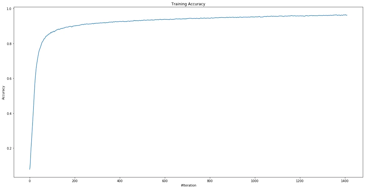
The average training accuracy is summarized below. As expected, accuracy surpassed 80% within the first 100 iterations and gradually improved thereafter.
The next step is to produce the prototypicality ranking described by the paper. I chose to produce the ranking by applying the Ensemble Agreement(AGR) proposed in the paper, which computes symmetric JS-divergence for each example among ten models’ predictions.
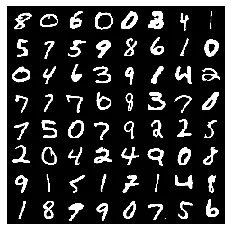
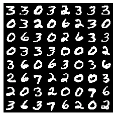
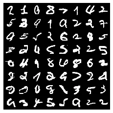
(Left: 64 random examples. Middle: top 64 typical examples. Right: top 64 atypical examples)
All examples were divided into ten chunks by their AGR scores, the first chunk being the most well-represented and the last chunk being the least well-represented. Their training accuracies are shown below.
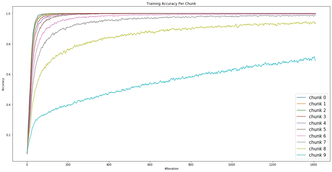
Interestingly, even the simplest neural network training inherently follows an implicit curriculum: learning begins with typical, well-represented examples and gradually progresses to more challenging ones. For instance, most well-represented examples (chunk 0) are almost entirely learned within the first 50 iterations, whereas the accuracy for chunk 9 improves at a much slower pace.
Why do neural networks learn the “easy” examples first
How does such a curriculum naturally emerge during stochastic gradient descent training? Why are examples with varying levels of prototypicality treated differently?
To explore this, I calculated the cosine similarity between the gradient of each individual example (from the evaluation step) and the average gradient across all examples. The plot below illustrates the results: the X-axis represents the number of iterations, and the Y-axis shows the average cosine similarity between example's gradient and the overall average gradient for the mini-MNIST dataset, for each chunk.
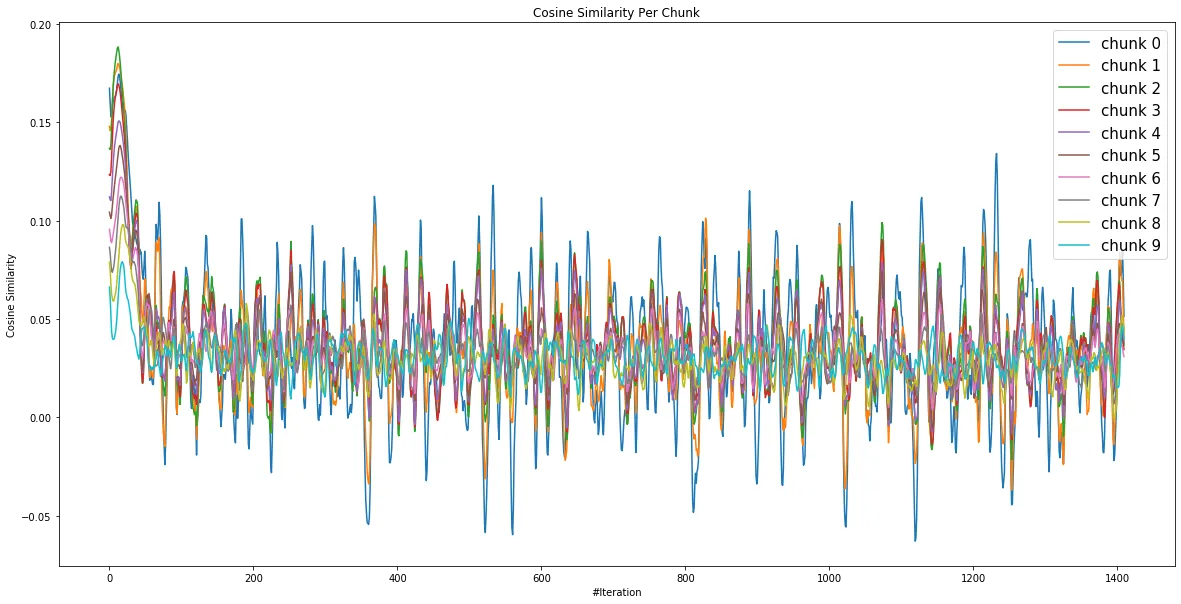
The results show that the most well-represented chunk has the highest cosine similarity score, particularly during the first 50 iterations. This aligns with the observation that these examples benefited the most from training and achieved higher accuracy more quickly.
On closer visual inspection, it’s evident that "well-represented" examples share many similarities, leading to more similar gradient vectors. When aggregated, these vectors form a stronger overall gradient direction, effectively dominating the gradient descent process.
Additionally, well-represented examples tend to have smaller gradients, as their associated losses are generally lower.
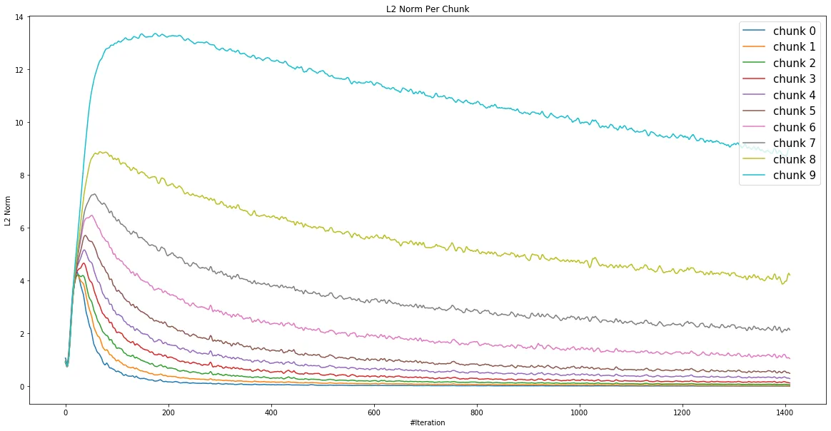
average l2 norm per chunk ranked by prototypicality
Well-represented examples are less prone to forgetting
In addition to the finding that examples of well-representation are learned faster, they are also less forgotten by the network once they’re learned. Here, I defined two new metrics in addition to the accuracy:
-
First Correct (FC): The percentage of examples for which the model achieves at least one correct classification up to and including the current iteration.
-
Last Mistake (LM): The percentage of examples for which the model makes no incorrect classifications from the current iteration onward, including the current iteration.
By definition, FC and LM are both monotonically increasing, and FC is always greater or equal to the actual prediction accuracy, LM is always less than or equal to the prediction accuracy.
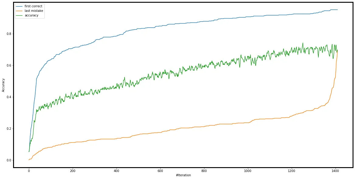
Using the definitions above, I created three plots for the top 10%, middle 10%, and bottom 10% of training examples ranked by AGR.
The blue line is FC, the green line is training accuracy, and the orange line is LM. The region between the FC and LM lines is particularly interesting, as it represents examples that the network has correctly classified before but is still struggling to fully learn.
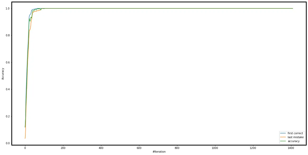
top 10% examples ranked by AGR
The plot above highlights the top 10% of well-represented examples that were learned very early in the training process and were never forgotten afterward! 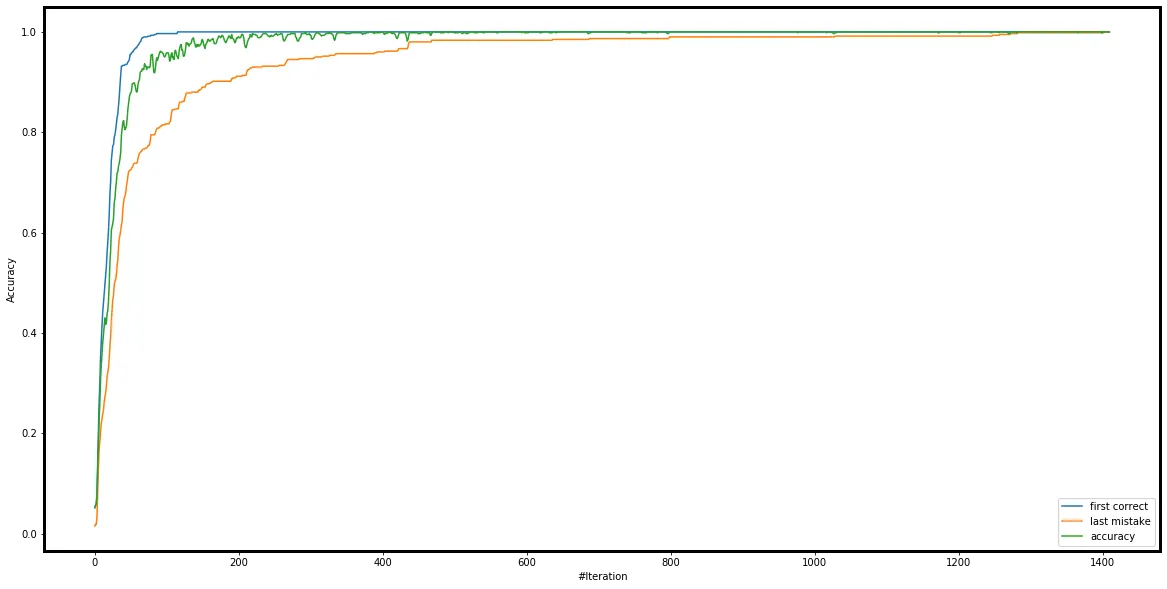
middle 10% examples ranked by AGR
As examples become less well-represented or more challenging, the envelope region expands, indicating that the network begins forgetting more of the early learned results as training progresses.
bottom 10% examples ranked by AGR
The plot above shows the accuracy for the bottom 10% of examples, along with the large region between FC and LM. This suggests that, although the network is making some progress, it fails to “secure” these learnings.
From the previous section, we know these examples are slow to learn because their atypical gradients are large and less aligned with the rest of the batch. But why do they also suffer from forgetting? Could this forgetting be caused by atypical gradients canceling each other out?
Visualizing individual example gradients
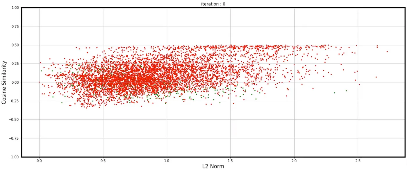
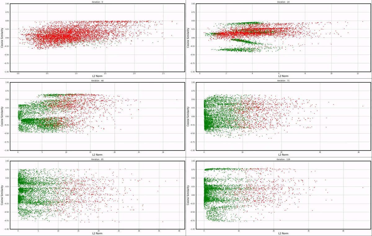
Using the individual gradients collected during training, I visualized them in a plot. The X-axis represents the gradient norm, while the Y-axis represents the cosine similarity between an example’s gradient and the average gradient of the dataset.
Each point corresponds to an example: green indicates correct classification by the network, and red indicates incorrect classification.
iteration 0
At the beginning (iteration 0), only a few examples (10% ?) were correctly classified by the randomly initialized network by luck. As the training progressed, more examples were correctly classified, and green points were moving to the left side of the plot because of low gradient norms, while the red points with large gradients moved to the right side. See here for the full video.
iteration 0 - 120
Training is chaotic, but still, we’re able to have some interesting observations:
Cluster of gradients
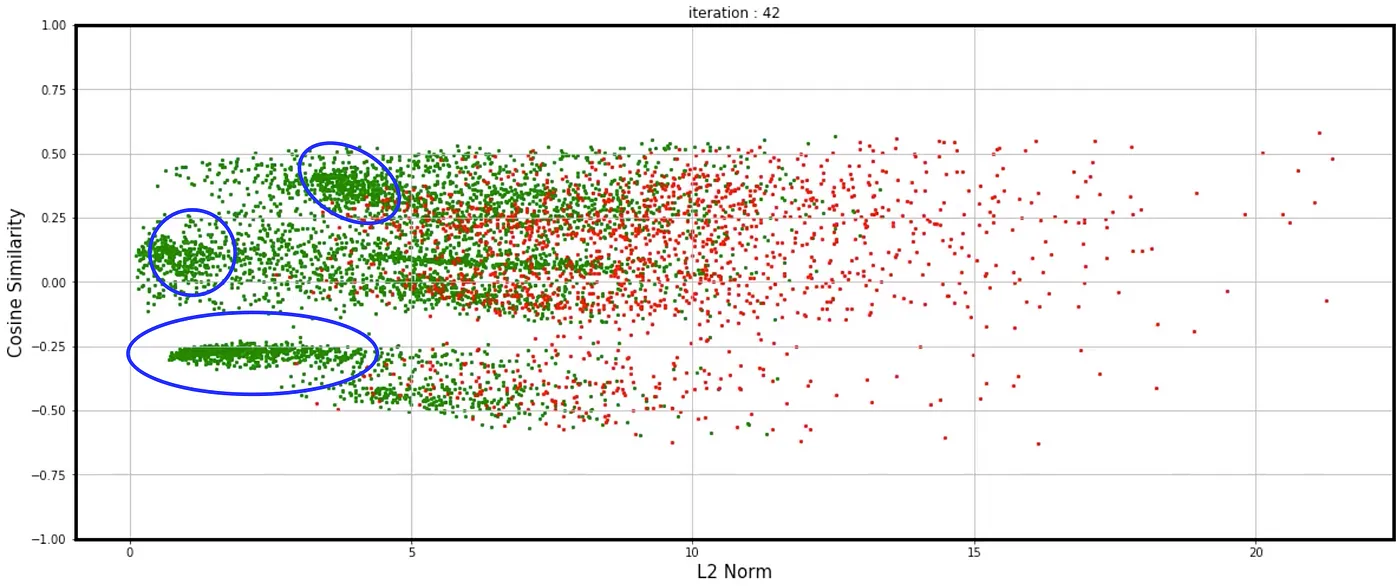
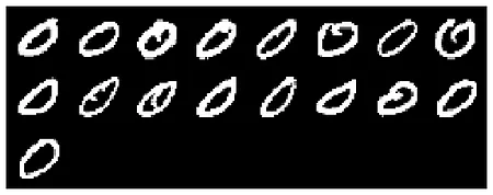
It’s evident that some examples’ gradients consistently move together, likely due to strong similarities among these examples. By identifying "cones" where all examples fall within a cosine similarity of 0.95 with each other, we can isolate clusters. This approach allows us to zoom in on small groups of examples, revealing distinct styles and nuances between them, even within the same class.
Here are some example clusters identified by similar gradients:


Oscillation and examples in contention
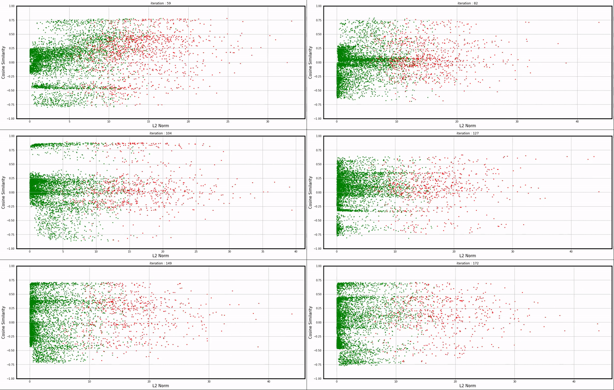
Looking closer, particularly after iteration 30, we can observe some clusters oscillating between positive and negative cosine similarity.
My initial hypothesis is that this oscillation arises from two groups of examples with gradients that counteract each other. Gradients from group 1 are initially larger, allowing them to dominate the batch and benefit from stochastic gradient descent, leading to improved accuracy for these examples. Simultaneously, another group (group 2) is negatively impacted by the gradient updates, causing their accuracy to drop and their losses and gradients to grow. Eventually, group 2's gradients surpass those of group 1, shifting the balance and allowing them to dominate the batch. This back-and-forth process repeats, resembling the dynamics of rotating binary stars.
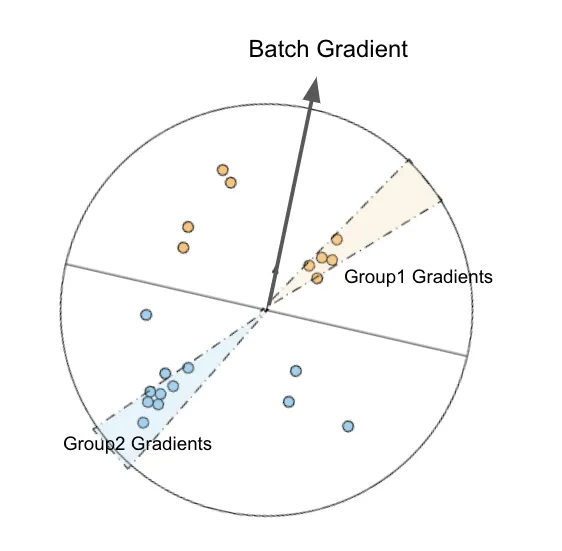
We could find those clusters using the “cone” cover technique mentioned above. For each cluster, we can also find examples learning against them by identifying examples under -0.95 cosine similarities. This reveals example clusters that are “fighting” against each other during training; This is interesting as it can give us insights into what kind of examples the network is struggling to learn and visually examine.
Contention between "2"s and "1"s:
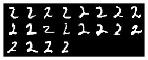

It makes sense the network confuses these two groups of examples from a visual perspective, and we can see symmetry in the cosine similarity plot and accuracy plot where one group’s gain is another group’s loss.
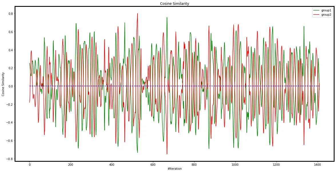
cosine similarly between each group and the average gradient of the entire mini-MNIST
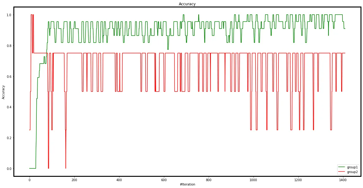
average prediction accuracy of each group
Contention between "2"s and "6"s:


This observation is intriguing, as the 6s (right) resemble mirrored versions of the 2s (left). This similarity might suggest that the network struggles to learn distinct and accurate representations for both digits.
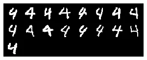
Contention between "9"s and "4"s:
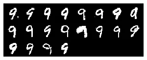
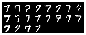
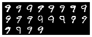
Contention between "7"s and "9"s:
Visualize gradients in networks with more than one hidden layer
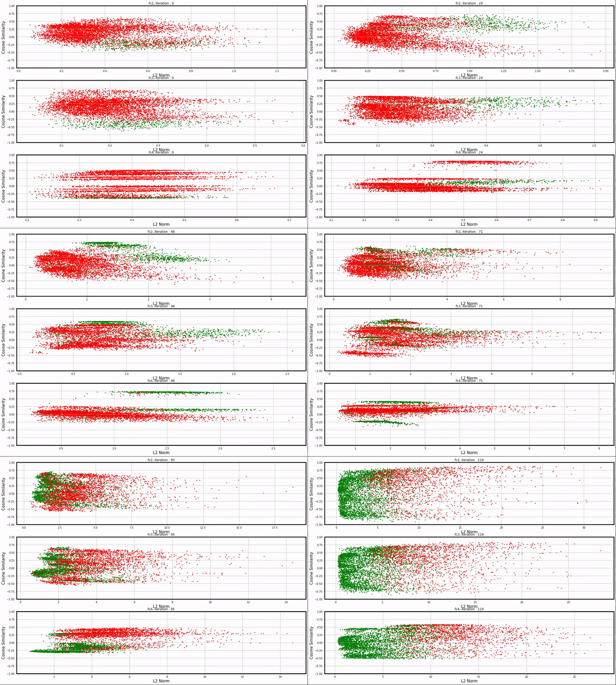
All these visualizations above are from networks with single hidden layers; we could apply the same visualization technique to networks with slightly more complicated architecture as well.
I trained a network with four fully-connected layers (fc1: 28*28 -> 32, fc2: 32 -> 16, fc3: 16 -> 10, fc4: 10 -> 10)
and applied the same visualization technique on fc2, fc3, and fc4. See here for the full video.
Conclusion
The simplest neural network training demonstrates an implicit curriculum: well-represented examples are learned much faster and are less likely to be forgotten. The per-example gradient visualization uncovers fascinating phenomena, such as gradient clusters and the contention between two groups of examples that the network struggles to learn.
While this experiment focuses on a very basic neural network, I hope it provides insights and sparks ideas about the complex and often chaotic training dynamics of deep neural networks.
Acknowledgments
I would like to thank Jason Yosinski, Rosanne Liu, and Sara Hooker for their guidance and support, and the ML Collective community for the comments and discussions.